Antwerp QC, Much of Belgian Core, Leaves Competitive Quidditch

This is the first installment of a season-long exploration into the topic of how community teams and college teams stack up by numbers. Alejo Enriquez, Joshua Mansfield and Shane Hurlbert will be conducting all research on the topic.

If you are a regular reader of The Eighth Man, you are no doubt familiar by now with the discussion in the quidditch community on the topic of college teams and community teams and whether there is a growing imbalance between the two, and what to do about it if there is one. My own team captain, the esteemed Augustine Monroe, even wrote a piece not long ago addressing this potential disparity and calling for action. Yet the inertia of the current system appears potent, as it so often is, and so to effect real change there has to be a consensus of some kind that change is needed. This piece is not designed to persuade anyone of anything with intent, but rather, to present the facts as they are with cold-hard, uncaring numbers, and allow you to come to your own conclusions about what they mean (with some minimal guidance on my part, of course).

PART 1: STATISTICS
In this piece I will be presenting a few stats as they are understood in sports, meaning descriptive numbers. However, I will also be using statistics as scientists such as myself are accustomed to using. I will briefly describe how this works in this space for your edification. Those of you who are already familiar with statistical tests are advised to skip the next two paragraphs because I will be describing them in overly broad and vague terms and you may be bored and/or irritated by it.

A statistical test works by supposing that two numbers (or groups of numbers or ratios or what have you) may in fact originate from the same source, then finding the probability that this is true. In essence, sample size and amount of variation are compared using headache-inducing formulas that no one memorizes to show how likely it is that the differences are in essence a fluke. If I were to flip a coin three times and get heads twice I would not experimentally see the “true” ratio is 50/50, but a statistical test would in fact show that there’s a reasonable probability that the true ratio is in fact 50/50. If I were to flip the same coin 300 times and get 200 heads and only 100 tails, something strange is clearly going on with this coin, and the statistical test would reveal as much.

The most important thing when looking at a statistical test is the p-value. It is the probability that the groups of interest are actually from the same source. Scientists and statisticians usually use p=0.05 (5 percent likely to have happened by chance if the groups are actually from the same source) as the arbitrary cutoff point for declaring that there is a “significant” difference between the two groups. In the example above, a statistical test on three coins flips will not find a significant difference between the experimental probability of getting heads (66.7 percent) and the “true” value of 50/50, while a statistical test on the 300 coin flips would find a very strong statistical significance between the experimental probability of heads (66.7 percent) and the theoretical probability of 50 percent.

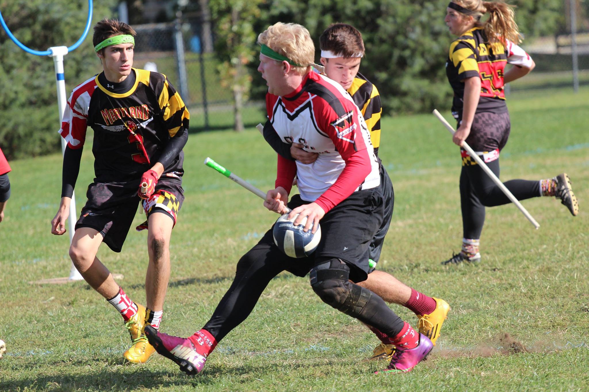
Credit: Loring Masters

PART 2: METHODS
For this analysis I am using USQ 2015-16 official games only. My available data set as of this writing is dated October 28, and, assuming I am not metaphorically run out of town, I will continue to run the latest data with the same techniques presented here. Additional disclaimer: I am using the Crimson Elite’s game-result scores and not the forfeiture scores, since (A) the sample size is small enough that this might contaminate the results, and (B) the real question everyone is worrying about is on-field product and not the email-checking abilities of team managers, which is not anticipated to be a big factor at USQ Cup 9.

At the time of this writing, there are 247 games played with verified public-record scores. Each of these games has been loaded as a separate entry into a personal-use SQL database along with the identity of each team (gratitude owed here to my MLQ colleagues for their help with the game entry). I manipulated the data using SQL code, and then exported to Excel for statistical analysis.

In advance of any questions or comments I will also mention that since Wolf Pack Classic was not included in the data set, we do not yet see Lone Star Quidditch Club, University of Texas and many other prominent Southwest teams represented in this analysis at all, nor most of the major West teams since their season has not begun in earnest either.

PART 3: CVC WINS
Of the 247 games in the current iteration of the dataset, only 74 are games played between a college team and a community team, which means these are the games I focused on. Since the concern everyone has is that community teams may ultimately outclass college teams, community teams playing against each other are not of interest for this statistical project.

Of these 74 games, 50 were won by community teams with 24 going to college teams. The first statistical test I employed is called a binomial test. The binomial test is a statistical test like for the coin flips described above, asking “are these results consistent with the hypothesized probability?” I tested the hypothesis that the probability of a community team beating a college team was 50 percent, and the binomial test result was p=0.00169. That means that there is less than a 2 out of 1000 chance that college and community teams, on the average, are equally likely to win. This is considered a statistically significant result.

INTERMISSION: LIES, DAMN LIES, AND STATISTICS
Numbers have a very fascinating way of not convincing people of anything. “So what, what does this even mean” is a valid question, but there are valid answers to be found here. If we truly care about this sport, we must come to grips with the reality that is occurring right now. Right now, community teams have beaten college teams two out of every three times they have played, and this is not simply by chance.

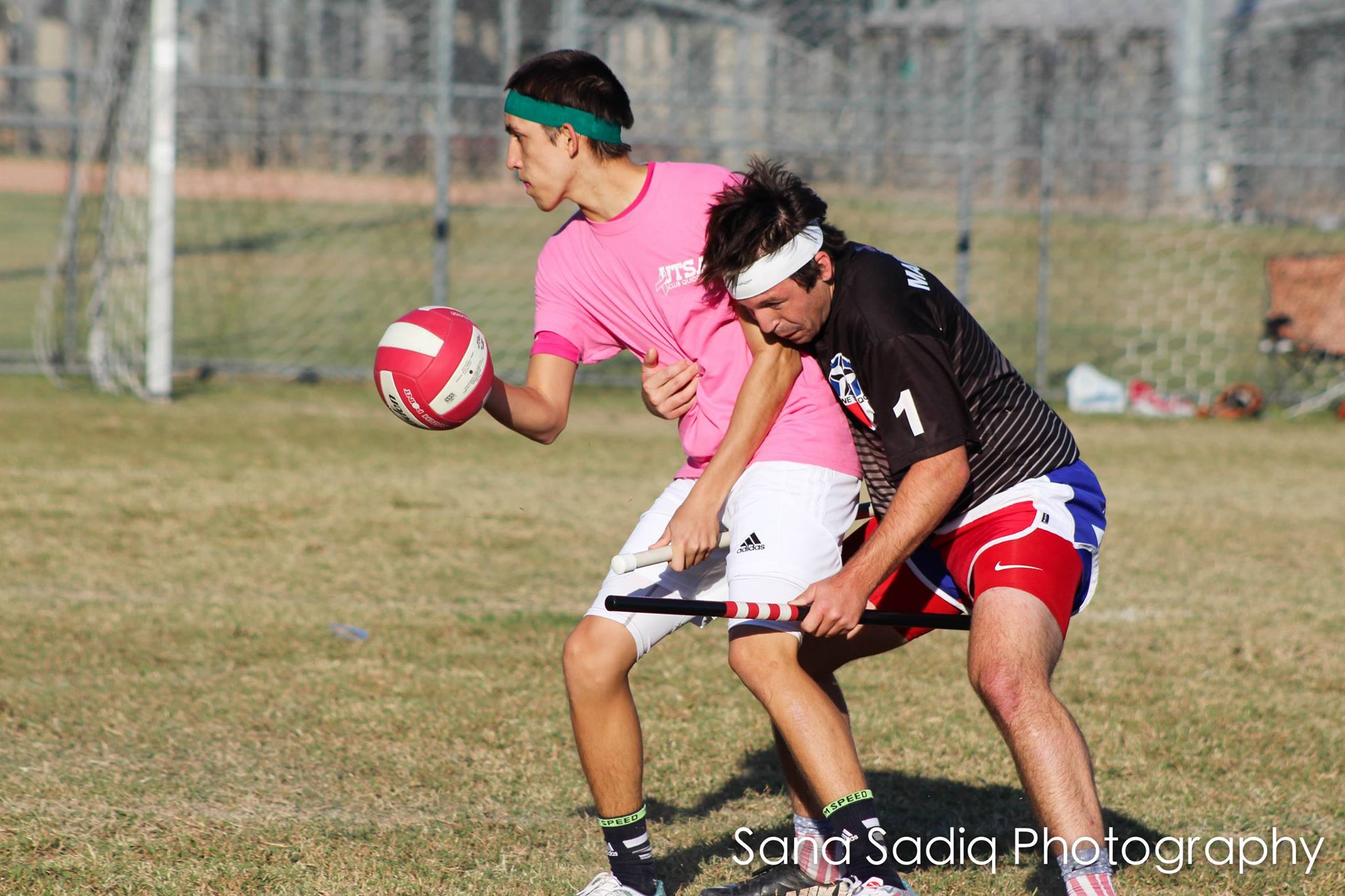
Credit: Sana Sadiq

PART 4: POINT DIFFERENTIAL
I calculated the point differential for each game between a college team and a community team and sorted them into two piles: the point differentials for games when a college team won and when a community team won, and then I compared them. To do this, I used a Student’s T test, which compares two piles of numbers and asks if they actually have the same overall average. To this question I got another “LOL NO” in the form of p=0.00393, meaning it’s less likely than one in 250 that college teams are winning by the same margin as community teams (for the record, the averages in question are 104.6 average winning point differential for community teams versus 62.5 for college teams).

Next, I calculated each team’s net point differential (meaning if Team A wins a game 100-60 and loses another 50-40, their net point differential is now 30, after the +40 and the -10 are combined). Point differential is generally accepted as an indicator of how dominant a team has been during its games, and for this reason I ran this test on all games, not only the college versus community games. I did this because I anticipated the argument that a few dominant teams might be skewing the result, and sure enough, QC Boston and Rochester United sported the only net point differentials above 100 per game (141.7 and 122.5 net average point differential per game).

When I ran a T test on the college teams’ net point differentials versus the community net point differentials I found p=0.02621, meaning that there is less than a 3 percent chance that equal groups of teams would produce these point differentials. When I ran a rank order T test (which reduces the effect of outliers) the p-value increased but was still showing statistical significance at p=0.04542. This in particular is somewhat damning, as a rank order test typically removes the effect of having a few large numbers at the top skewing the results. While there are certainly fantastic college teams (Baylor is rocking a net average point differential of 100.0) and some hapless community teams (Crimson Fliers tied the Boise State Thestrals with a -112.5 net average point differential), the trend is clearly showing that if you choose a random community team and a random college team, on the average the community team WILL have a higher win percentage and point differential than the college team.

PART 5: ECOLOGICAL ANALOGY
In ecology, the study of the way animals and plants live, there are understood to be two categories of reproductive strategies: r-selection, which favors a rapid population growth, and K-selection, which favors stable, long-lived organisms that reproduce less frequently but with greater success. I bring this up because I feel this is a highly analogous situation to what we’re seeing in the growth of the sport of quidditch.

R-selected organisms are generally understood to be more successful when first populating a new area due to a high level of recruitment. One weed can quickly become hundreds, and they can reproduce as quickly as they are eaten and stepped on. Trees, on the other hand, take time to grow and do not reach maturity for a long time. Trees and other K-selected organisms, however, perform much better in a stable, long-term environment with fewer disturbances. Ultimately, a field, if left undisturbed and allowed to flourish, will eventually become overrun with trees better able to access sun and water than smaller, faster-growing weeds, and if they are permitted to continue competing directly, the weeds will eventually die out.

For a new sport starting out, the most successful teams will be the ones with the highest recruitment of new players, and there is literally no better source of young adults with a lot of energy and some minimal amount of time and money than in college. College teams thus have had (and will continue to have) a recruitment advantage, and if the entirety of a quidditch player’s career lasted three years, college teams would be dominating into the foreseeable future. What we’re starting to see, however, is that the pool of experienced players is increasing, and these players will naturally collect into community teams since many college programs have stringent limitations on who can play for their club sports. We’re beginning to see a shift in the balance of power, where K-selected community teams are able to attract and retain enough players to compete with the higher recruitment ability of college programs.

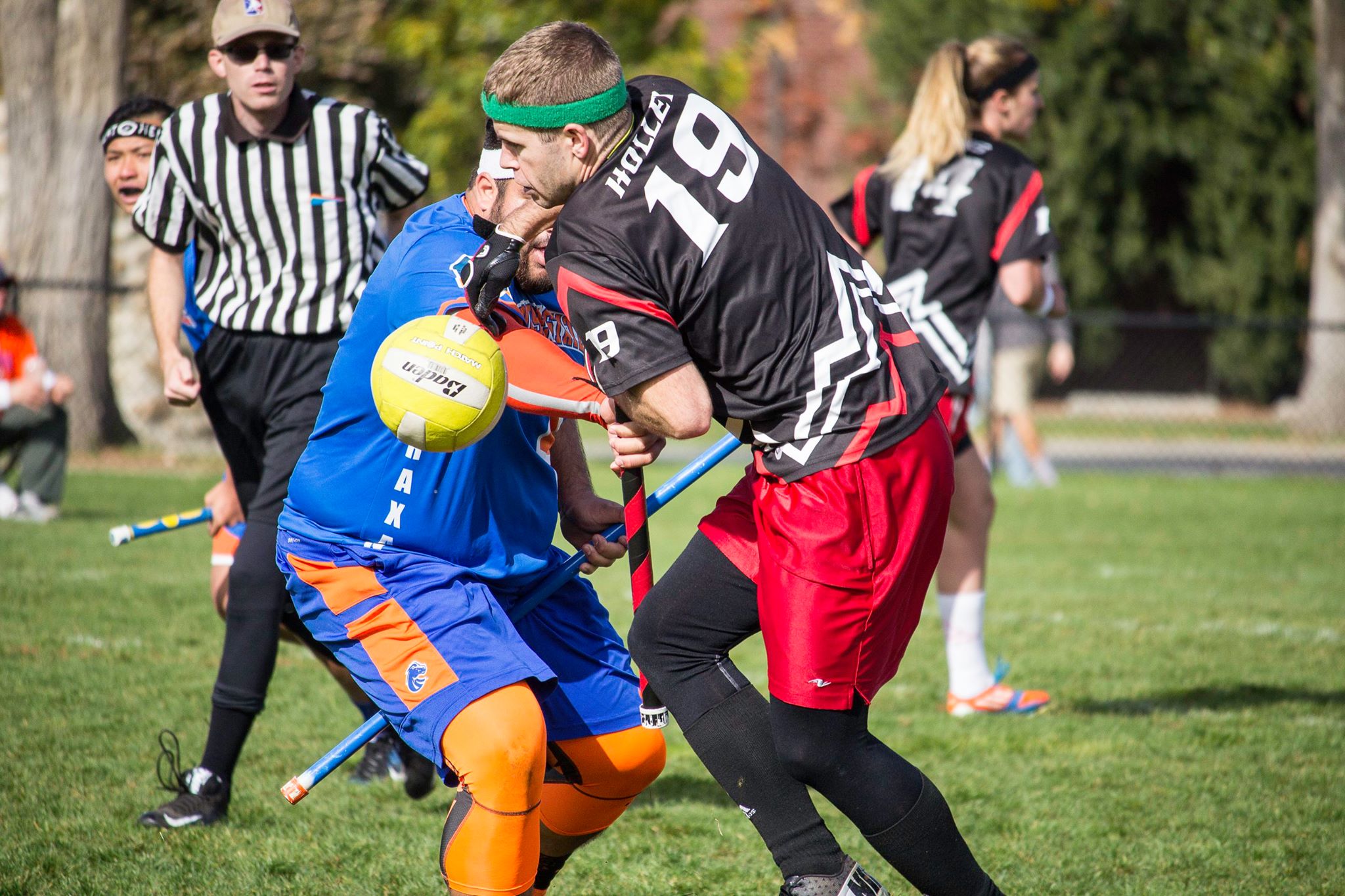
Credit: Lang Truong

I am not proposing to have all (or any) of the policy answers to this situation, nor am I attempting in this space to project these numbers into the future. I will point out that in the sport of gridiron football, college teams used to play against semi-pro and professional teams, but the NFL’s ability to cull the top college players and retain them for years and even decades has put its level of play far above any college program’s wildest dreams (sidenote: the Super Bowl winner used to play a college all-stars team in an exhibition show, which sounds like something that was probably an awesome idea at the time and probably was ended for really, really good reasons). If we, as a quidditch community, wish for our sport to be a long-term success story, then we must face the facts that eventually some teams will have many more experienced players than others. Ultimately, we must decide how to balance our natural desire not to restrict who plays whom with our natural desire not to see 300*-0 beatdowns on a regular basis, because these are mutually incompatible goals.

Archives by Month:

Archives by Subject:

Categories